Galerkin Transformer: A One-Shot Experiment at NeurIPS 2021

WARNING: very lengthy read!

Takes about 23 minutes if the mathematical expressions are taken for granted.

Prologue: random babbling from a newbie

Recently I wrote my first paper on machine learning: (Cao, 2021) as a fun yet challenging side project. The open-source repository containing the codes is here:

https://github.com/scaomath/galerkin-transformer.

Being a complete newbie to this field, I am stupidly crazy enough to submit this paper to NeurIPS 2021…thanks to my mentor’s encouragement.

The title was pretty catchy, I thought, as searching “Galerkin Transformer” would have the paper’s arXiv link on top. As an amateur mathematician, this title would indicate that this is more like a “having fun not aiming for publication” type of paper. Then, I saw some other “apparent” NeurIPS submissions (using the NeurIPS $\LaTeX$ template) with titles like “Anti-Koopmanism” , “Max-Margin is Dead, Long Live Max-Margin!”, “You Never Cluster Alone”. Bazinga! Unquestionably, these CS people are really serious about this.

The paper itself is semi-theory, semi-experiment. I feel like even though everyone is using Transformers because Attention is all you need¹, even for CV tasks, saying “mathematics behind the attention mechanism is not well understood” is even a bit of an understatement, because there are barely any rigorous theoretical foundation to explain why attention would work in such a magical way mathematically.

So, in the rest of this blog post, in a causal casual manner with some semi-seriousness in the mathematics behind, I will introduce our tiny attempt in (Cao, 2021) on rethinking Transformers with some serious math that I am familiar with:

• An attempt on explaining the approximation capacity of the attention mechanism for the first time using the Galerkin method from the approximation theory in Hilbert spaces.

A newbie’s attempted tour at NeurIPS 2021 submission

More interestingly, NeurIPS 2021 decided to run an experiment of this author survey:

We are inviting all authors of NeurIPS submissions to fill out a very short (<5 minutes) survey between now and June 11, 2021. The purpose of this survey is to evaluate how well authors’ expectations and perceptions of the review process agree with reviewing outcomes.

All authors are asked to estimate the probability that each of their papers will be accepted in the NeurIPS 2021 review process. Authors who submitted more than one paper will additionally be asked a second question: to rank their papers in terms of their own perception of the papers’ scientific contributions to the NeurIPS community.

After carefully studying some past rejections that are made public on Open Review, I filled the most statistically making-sense number: 20%, which is the average acceptance rate at NeurIPS. I believe, after the survey results become available in the future, there will be sensible authors like myself, and there will be optimists who believed their work is fundamental but hardly incremental. The results will probably be seriously skewed toward both 0%, 20%, and the other end of the spectrum: 80%, 90%, 95%.

Attention needs softmax normalization

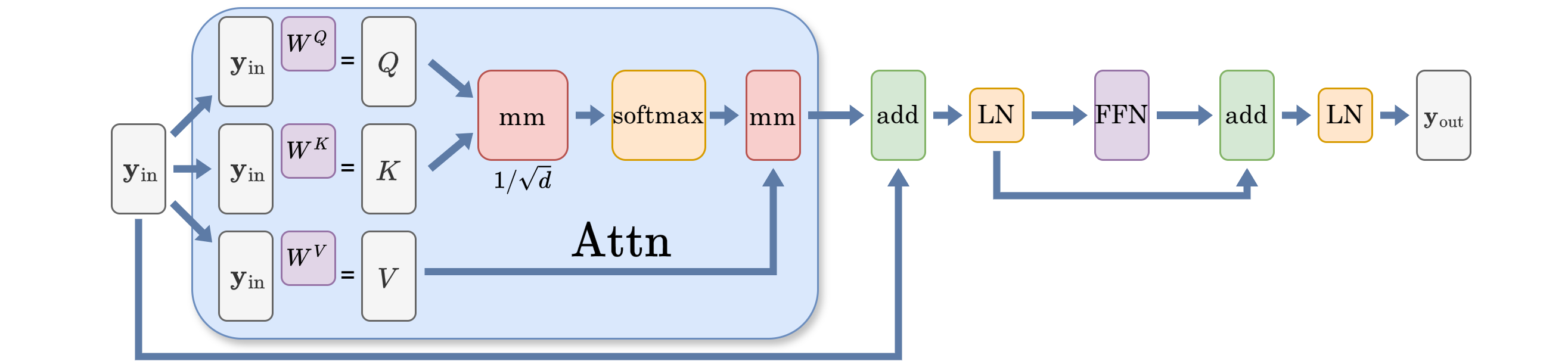
The self-attention operator is mathematically defined as follows: $\mathbf{y}\in \mathbb{R}^{n\times d}$ is the input latent representation, query $Q$, keys $K$, values $V$, along with projection matrices $W^{\diamond}$, $\diamond\in {Q,K,V}$

\[W^Q, W^K, W^V \in \mathbb{R}^{d\times d}, \\ Q = \mathbf{y} W^Q, \quad K = \mathbf{y} W^K,\quad V = \mathbf{y}W^V.\]

The scaled dot-product attention is:

\[\text{Attn}_{\text{softmax}} (\mathbf{y}) := \text{Softmax}\left(d^{-1/2}QK^\top \right)V.\]

The full attention is: for $\sigma(\cdot)$ a pointwise universal approximator (feedforward neural net in this case)

\[\operatorname{Attn}: \mathbb{R}^{n\times d}\to \mathbb{R}^{n\times d}, \\ \mathbf{z} = \operatorname{LayerNorm}( \mathbf{y} + \text{Attn}_{\text{softmax}} (\mathbf{y} )) \\ \mathbf{y} \mapsto \operatorname{LayerNorm} \left(\mathbf{z} + \sigma(\mathbf{z})\right). \tag{A}\label{eq:A}\]

In many papers on the interpretation of the self-attention mechanism in Attention is all you need¹, including some recent attempts, making analogies with a “kernel interpretation”²³, or say linking the $\text{Softmax}(QK^T)V$ as a learnable kernel map is a common practice. $\text{Softmax}(QK^T)$ is described as a similarity measure for each position’s feature vector (learned embeddings of the tokens) with that of every other position. Some notable linearizations⁴⁵⁶ of the softmax-normalized Transformers are exploiting this interpretation.

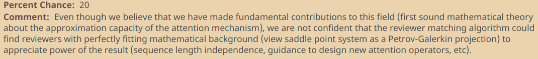
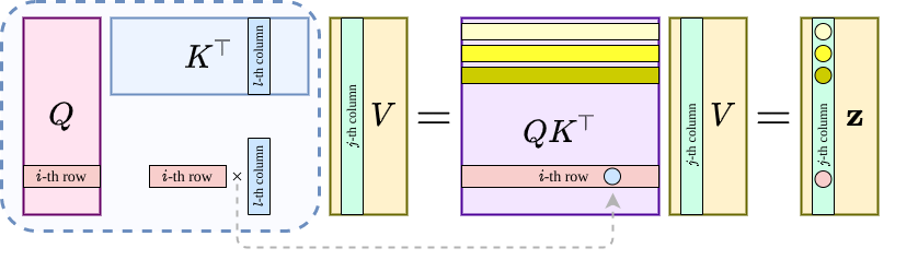
I thought, the life would be infinitely easier if it were softmax-free, and we change the interpretation from row-wise to column-wise. So let us do it! The reason is simple, while each row represents the learned embeddings from the tokens of each position, each column can be viewed as a basis function sampled at the grid points from the positional encodings!

An attempt to improve the attention mechanism based mathematical intuition

Now assume that $Q,K,V$’s $j$-th column as (separate) functions $q_j(\cdot)$, $k_j(\cdot)$, $v_j(\cdot)$ sampled at physical locations $x_i\in \mathbb{R}^m$ for $i=1,\dots, n$, along with $z_j(\cdot)$ denoting that of the output of the scaled dot-product. Then, $(QK^T)V$ along with some caveats on the skip-connections, the attention without softmax becomes the Fredholm equation of the second kind:

\[\text{For}\; j=1,\cdots,d,\;\text{ and } x\in \{x_i\}_{i=1}^n, \\ \delta_j^{-1} v_j(x)\approx z_j(x) - \int_{\Omega} \kappa(x,\xi) v_j(\xi) \mathrm{d} \xi,\]

with $\kappa(x,\xi):=\zeta_q(x)\cdot\phi_k(\xi)$ for feature maps $\zeta_q(\cdot), \phi_k(\cdot): \mathbb{R}^m \to \mathbb{R}^{1\times d}$.

Interpreting the attention mechanism as an integral is not new, for example the integral on group has been exploited in LieTransformer⁷. Nevertheless, introducing the integral into the picture invites a more interesting interpretation for the linear variant without softmax: $Q(K^TV)$ can be viewed as a Petrov-Galerkin projection (if we treat $Q,K,V$’s columns as independent functions):

\[\text{For}\; j=1,\cdots,d,\; \text{ and } x\in \{x_i\}_{i=1}^n, \\ z_j(x) := \sum_{l=1}^d \mathfrak{b}\big( k_l, v_j\big) \, q_l(x), \tag{$*$}\label{eq:attn-g}\]

where $\mathfrak{b}(\cdot,\cdot)$ is a bilinear form defined on infinite dimensional Hilbert spaces, yet in action evaluated for discrete approximations. To help us understand, we can refer to the following two figures to see how the life becomes much easier without softmax.

Now to bridge the expression \eqref{eq:attn-g} for linear attention (without softmax) with something we are familiar with, we can further think about $QR$-factorization, or even a projection in a set of orthogonal basis ${q_j(\cdot)}_{j=1}^d$:

\[\min_{a_i}\Big\| f - \sum_{i=1}^d a_i q_i(\cdot)\Big\|^2_{L^2(\Omega)}. \tag{F}\label{eq:fourier}\]

The solution is, not surprisingly, a projection, if we assume that ${q_j(\cdot)}_{j=1}^d$ is further normalized by its inner-product induced norm (think of instance normalization with a further $1/\sqrt{n}$ weight).

\[z(x) := \sum_{l=1}^d \Big(\int_{\Omega} f(\xi) \, q_l(\xi) \mathrm{d} \xi\Big)q_l(x), \tag{P}\label{eq:fourier-p}\]

The simplest example would be letting $\Omega = [0,2\pi]$ and $q_j(x) = \sin(jx)$ and $\cos(jx)$, then \eqref{eq:fourier-p} is just a Fourier series partial sum approximation for a function in $L^2(\Omega)\cap C^0(\mathbb{S}^1)$ and a special case of the one in \eqref{eq:attn-g}.

Inspired by this interpretation, the following Galerkin-type simple attention operator is proposed:

\[\operatorname{Attn}_{\text{simple}}: \mathbb{R}^{n\times d}\to \mathbb{R}^{n\times d}, \\[3pt] \mathbf{z}= \mathbf{y} + \operatorname{Attn}_{\mathfrak{g}} (\mathbf{y}) \\[3pt] \mathbf{y} \mapsto \mathbf{z} + \sigma(\mathbf{z}),\]

no softmax, at, all. The layer normalization is done for the latent representations before doing the dot-product, just like the Fourier basis can be viewed to have a pre-inner-product normalization,

\[\text{Attn}_{\mathfrak{g}} (\mathbf{y}) = Q\Big(\operatorname{LayerNorm}(K)^T \cdot \operatorname{LayerNorm}(V)\Big)/n. \tag{G}\label{eq:attn-simple}\]

Operator learning

Now that a new attention is conceived, the question is:

Where do we set the stage for this new attention operator?

Even though some initial prototyping suggests promising results on the BLEU evaluation benchmarks on IWSLT14 (De-En) using fairseq (much faster training, for example), to myself, the operator learning problem related to Partial Differential Equations would be the natural choice. BTW the prototyping-debugging-improving cycle is too long for myself if opting for a big and arduous NLP problem.

Last year, my mentor sent me a blog post (in Chinese) about the Caltech ML group achieving a state-of-the-art performance using the so-called Fourier Neural Operator (FNO) to learn a PDE solution operator⁸. After reading it carefully, dissecting the codes, and re-implementing it myself, I was totally bowing to the feet of this awing approach as it beats previous methods by orders of magnitudes. Moreover, the implementation convinced me that the general Q/K/V approach in attention becomes the FFT->conv->iFFT. This change is a special and efficient linear variant of the attention mechanism, with $W^Q$ and $W^K$ non-trainable. As FFT or iFFT can all be viewed as a non-trainable change of basis through multiplying a Vandermonde matrix. In the original versions \eqref{eq:fourier-p} and \eqref{eq:attn-simple}, the weights for the (nonlinear) change of basis are all trainable.

Most importantly, the practice in FNO inspires us that

• Softmax is not necessary in either frequency or spacial domain.
• Treating the columns of the latent representation to exert operations upon, not rows (positions’ feature vector), is a promising approach.

Until recently (as of May 2021), the ML community started to appreciate this direction.⁹¹⁰.

Benchmarks

Well, what is the result? We considered the famous benchmark problem such as the following:

\[\begin{aligned} -\nabla \cdot (a\nabla u) = 1 & \text{ in } \;\Omega, \\ u = 0 & \text{ on } \partial \Omega. \end{aligned}\]

The operator to be learned is between the diffusion coefficient and the unique weak solution:

\[T: L^\infty(\Omega) \to H^1_0 (\Omega), \quad a\mapsto u.\]

This is to say: given the coefficient, a trained operator learner should be able to give the solution’s approximation directly from the coefficient.

The combination of the attention with FNO is crazily good, and it can solve the difficult inverse coefficient identification problem as well. As under the same parameter quota, in the Burgers’s equation benchmark, the 4 Galerkin attention layers+2 FNO layers model outperforms the one with 4 FNO layers by 4 times under the same lab condition (1cycle scheduler¹¹ of the same LR, 100 epochs). The common range of the mean evaluation relative error in $L^2$-norm is 1e-3 with the maximum being 1.7e-3. The benchmarks in the Darcy flow, together its inverse version, has dethroned the king (FNO) as well in terms of evaluation accuracy; the training of the Galerkin Transformer is slower than FNO despite theoretically being the same order of complexity.

Other than the neural operator structured networks proposed by the Caltech group, the next close competitor, DeepONets, is much worse…(c.f. Page 14, Figure 10 for that single instance having 3e-2 relative error). As the network in DeepONets resembled the additive attention in Neural Turing Machine (NMT), it is predictable that DeepOnets, despite having a structure heuristically conforming with the math, are harder to train due to the composition of multiple “difficult” nonlinearities such as tanh and sigmoids.

What can we prove? A Petrov-Galerkin projection.

The attention operator in either \eqref{eq:fourier-p} or \eqref{eq:attn-simple} is a nonlinear operator with respect to both its input and the trainable parameters. How can we bridge it to something like a Galerkin or Petrov-Galerkin projection (which are linear)? The answer is simple: we try to prove the approximation capacity in the following sense under a Hilbertian framework:

\[\min_{\theta}\| f - g_{\theta} \|_{\mathcal{H}} \leq \min_{v\in \mathbb{V}_h} \|f - v\|_{\mathcal{H}}. \tag{M}\]

This translates to: $g_{\theta}$, the approximator built upon the Galerkin-attention, has its approximation power on par with a Galerkin projection to an approximation subspace $\mathbb{V}_h\subset \mathcal{H}$.

This subspace $\mathbb{V}_h$ is the current one based on the latent representation, and during optimization, is dynamically changing. Yet, in a static view of a fixed latent representation, the attention mechanism has capacity to deliver the best approximator, a Galerkin-type projection, in the current approximation spaces.

Difficulties: bridging nonlinear mapping with a linear projection

One might ask: isn’t this trivial? Well, sort of, as \eqref{eq:fourier} is exactly the case when $\mathbb{V}_h :=\operatorname{span} \{ v_j(\cdot) \} $. However, upon closer inspection, it may not be that easy to mathematically lay this result in a crystal clear fashion. Here are the difficulties:

• Unlike the space setting in the Galerkin projection, the approximation subspaces represented by $Q/K/V$ are different.
• How to linearly combine the columns of $Q$ to get each column of the output $\mathbf{z}$ in \eqref{eq:attn-simple} depends on each column of the product $K^TV$. Yet it is not entirely clear that a certain column of $K^TV$ suffices to give the coefficients to yield a Galerkin or Petrov-Galerkin projection for any function $f\in \mathcal{H}$ as neither $Q/K/V$ are guaranteed to be of full rank, nor the surjectivity of the nonlinear inner product.

A simple example to illustrate the difficulty

In the context of any linear variant of attentions, $Q$ stands for values, $K$ for query, and $V$ for keys. Let us consider a simple example, where $\Omega=(-1,1)$, discretized by $-1=x_1<x_2<\cdots<x_n=1$. $Q$’s column’istic approximation space is made by the first two Chebyshev polynomials $\{1, x\}$, and those of $K$ and $V$’s are $\{a, bx\}$ and $\{c, dx\}$ for $a,b,c,d\in \mathbb{R}$ learnable. The actual columns are made by these functions’ evaluation at $\{x_i\}’s$ with $n$ fixed for a sample. Yet the sequence length $n$ can be changed in the operator learning pipeline. For an admissible $f\in \mathcal{H}$, the $L^2$-projection of $f$ onto $\mathbb{Q}_h := \operatorname{span}\{1, x\}$ is:

\[\Big(\text{Proj}\,f \Big)(x) := p_0 + p_1 x, \\ \text{ where } p_0 = \frac{1}{2}\int_{-1}^1 f(\xi)\mathrm{d}\xi, \; \text{ and }\; p_1 = \frac{3}{2}\int_{-1}^1 \xi f(\xi)\mathrm{d}\xi \tag{L}\label{eq:proj-linear}\]

When interpreting the columns of $K/V$ as functions sampled at grids, the dot-product of $K^TV/n$ becomes an approximation to an integral and it is easy to verify:

\[K^TV/n \approx \begin{pmatrix} \int^{1}_{-1}ac\, \mathrm{d}x & 0\\ 0 & \int^{1}_{-1}bd x^2 \mathrm{d}x \end{pmatrix},\]

In this case, upon a further simple check we can see that $K^TV/n$ has capacity to replicate the coefficients for a projection in \eqref{eq:proj-linear} by just multiplying with a vector.

However, what if $K$ and $V$’s columns are changed to the evaluations of $\{a, bx\}$ and $\{cx, dx\}$ at the grid points?

\[K^TV/n \approx \begin{pmatrix} 0 & 0\\ \int^{1}_{-1}bc x^2 \mathrm{d}x & \int^{1}_{-1}bd x^2 \mathrm{d}x \end{pmatrix},\]

Suddenly the capacity to replicate the coefficients in \eqref{eq:proj-linear} is gone! Because after multiplying this matrix to $Q$: the subspace represented by the columns of $Q(K^TV)$ has no constant function in it! The interested readers are welcome to verify it.

Of course, this is an over-simplification by letting:

\[W^Q = \begin{pmatrix} 1&0 \\ 0 & 1 \end{pmatrix}, \;\; W^K = \begin{pmatrix} a&0 \\ 0 & b \end{pmatrix} \;\; \text{ and } \; W^V = \begin{pmatrix} 0&0 \\ c & d \end{pmatrix},\]

but you get the idea.

Proof: a saddle point problem in Hilbert spaces

Through the technique of my own expertise (mixed finite element), we can show that $Q(K^TV)$ has capacity to replicate a Petrov-Galerkin projection, provided that the following holds:

There exists a surjective map from the key space ($V$ in the linear attention) to the value space ($Q$ in the linear attention).

If some of us are interested in the details please refer the Appendix D in the paper.

Using a layman’s language to translate the mathematical meaning of the proof for the linear attention, it is:

For the best approximator (Petrov-Galerkin projection) in the value space, there exists at least one key to match an incoming query to deliver this best approximator.

Written in the form of an inequality:

\[\min_{\theta} \|f- g_{\theta}\|_{\mathcal{H}} \leq c^{-1} \min_{q\in \mathbb{Q}_h} \max_{v\in \mathbb{V}_h} \frac{|\mathfrak{b}(f_h - q, v)|}{\|v\|_{\mathcal{V}}} +\min_{z\in \mathbb{Q}_h}\|f-z\|_{\mathcal{H}}, \tag{C}\label{eq:est-galerkin}\]

where $c$ is the constant in the Ladyzhenskaya–Babuška–Brezzi inf-sup condition on the discrete approximation space:

\[\|\mathfrak{b}(q, \cdot)\|_{\mathbb{V}_h'} = \sup_{v\in \mathbb{V}_h} \frac{\left|\mathfrak{b}(q, v) \right|}{\|{v}\|_{\mathcal{V}}} \geq c \|q \|_{\mathcal{H}}\]

The inf-sup condition is applied for $q$ being an actual residual $f_h - q$ in \eqref{eq:est-galerkin}, it is equivalent to a saddle point problem if we want to minimize this residual:

\[\left\{ \begin{aligned} \langle w, v\rangle_{h} + \mathfrak{b}(p, v) & = \langle u, v\rangle_h, & \forall v\in \mathbb{V}_h, \\ \mathfrak{b}(q, w) &= 0, & \forall q \in \mathbb{Q}_h. \end{aligned} \right.\]

This saddle problem’s solution (best approximator as a Petrov-Galerkin projection) aligns exactly with $Q(K^T V)$ (with an updated set of projection matrices), without softmax.

Why Transformer has great scalability toward the sequence length

If $c$ can be proved to be sequence-length independent, then Galerkin Transformer’s approximation power is independent of the sequence length. Rather, the approximation power depends on d_model, i.e., how many basis functions we are willing to pay to approximate an operator’s responses on a subset. A perfect bridge between the operator theory and the (linear) attention mechanism without the softmax.

As I myself have done this little side project and return to my own field in the near future (maybe one more work on a multilevel Transformer exploiting the subspace correction nature of the residual in the attention mechanism), it is not surprising if with some slight chance the ML community find out the significance of this proof exploiting the surjectivity of the key-to-value map, in 1 or 2 years, there will be things like “Sobolev attention”, “Differential attention”, “Chebyshev attention”, attention using other integral transforms.

The One-shot Experiment

Before submitting the full manuscript to NeurIPS 2021, there was a huge bomb dropping by someone pretty established in the ML field by calling his own NeurIPS oral paper bullshit:

Please Commit More Blatant Academic Fraud by Jacob Buckman, https://jacobbuckman.com/2021-05-29-please-commit-more-blatant-academic-fraud

After a careful thought and having studied the reviews of several rejected papers on Open Review with technical proofs, I decided to run a one-shot experiment, in that there are several technical “traps” in the paper.

Continuous in continuum, stable in discrete

For people unfamiliar with the approximation of operator equations in the Hilbertian setting, the biggest confusion, after following the train of thought, is probably:

• The key-to-value map is defined using a bilinear form. This bilinear form is defined on two infinite dimension Hilbert spaces, but why the paper only shows its lower bound on the discrete approximation spaces?

The answer is a long one.

Before writing the paper, I read the reviews on one of the first papers³ trying to explain the approximation capacity in a mathematical rigorous manner using the Mercer kernel. Their proof was mainly porting the one in an early seminal work¹² to the setting of Banach spaces. Judging by the timing of their arXiv submission, it is safe to assume that they have submitted their work to NeurIPS 2021 as well (despite not using the $\LaTeX$ template).

In the Open Review page of their ICLR 2021 submission, reviewer 1 raised this key insightful question:

Another weakness in the argument is the fact that the kernel changes with every step of stochastic gradient descent. Namely, the parameters $W^Q$ and $W^K$ are updated and that changes the kernel function. As a result, training of Transformers does not operate in a single Reproducing Kernel Banach Space.

This is one of the major concerns the authors of the Mercer kernel paper did not answer directly with a clear argument. The answer in fact is kinda simple in the context of the operator learning:

Even though Transformer offers sequence-length invariant performance (model trained on $n=512$ can offer the same evaluation error on $n=512$ or $n=2048$), for a single sample, the approximation offered is through a discrete space with $n$ grid points. Thus, the theory can be formulated with dynamically changing approximation spaces but a single underlying Reproducing Kernel Banach Space.

For example, the space of the continuous piecewise linear functions sampled at $n$ grid points of $\Omega$, no matter how big that $n$ is, is a subspace of $L^2(\Omega)$. The approximation for each single sample is done at a discrete level. The approximation spaces are dynamically updated through optimization, but the underlying infinite dimensional Hilbert spaces ($L^2$, $H^{1+\alpha}$, etc, or even Banach spaces like $L^{\infty}$) are not changing!

I felt like it was a missing opportunity for the Mercer kernel paper, as the approximation theory is branded in an infinite-dimensional setting. As the approximation power of the Transformer architecture is still bounded to a finite dimensional subspace, limited by d_model which is the number of basis functions in our “column-oriented” interpretation.

Epilogue

NeurIPS 2021 committee decided to put a checklist near the end of the submission template:

The NeurIPS Paper Checklist is designed to encourage best practices for responsible machine learning research, addressing issues of reproducibility, transparency, research ethics, and societal impact.

Personally, I really like this checklist. It guided me through preparing the paper, and taught me that the following good practices in ML research:

• Acknowledging other people’s assets (code, dataset);
• Presenting an ML research with reproducible/replicable codes and instructions;
• Reporting error bars/bands with respect to different seeds.

Inspired by this checklist, as well as the acknowledgement in a recent paper I read⁷, I thanked everyone who enlightened me in the course of this little side project, even if it was just a one liner comment in a causal casual conversation.

Bibliography

1. Cao, S. (2021) “Choose a Transformer: Fourier or Galerkin,” in 35th Conference on Neural Information Processing Systems (NeurIPS 2021). Available at: https://openreview.net/forum?id=ssohLcmn4-r.

   @inproceedings{Cao2021transformer,
     title = {Choose a Transformer: Fourier or Galerkin},
     author = {Cao, Shuhao},
     booktitle = {{35th Conference on Neural Information Processing Systems (NeurIPS 2021)}},
     year = {2021},
     primaryclass = {cs.LG},
     arxiv = {https://arxiv.org/abs/2105.14995},
     code = {https://github.com/scaomath/galerkin-transformer},
     url = {https://openreview.net/forum?id=ssohLcmn4-r},
     note = {http://scaomath.github.io/assets/pdfs/gt_poster_neurips2021.pdf}
   }

   In this paper, we apply the self-attention from the state-of-the-art Transformer in Attention Is All You Need for the first time to a data-driven operator learning problem related to partial differential equations. An effort is put together to explain the heuristics of, and to improve the efficacy of the attention mechanism. By employing the operator approximation theory in Hilbert spaces, it is demonstrated for the first time that the softmax normalization in the scaled dot-product attention is sufficient but not necessary. Without softmax, the approximation capacity of a linearized Transformer variant can be proved to be comparable to a Petrov-Galerkin projection layer-wise, and the estimate is independent with respect to the sequence length. A new layer normalization scheme mimicking the Petrov-Galerkin projection is proposed to allow a scaling to propagate through attention layers, which helps the model achieve remarkable accuracy in operator learning tasks with unnormalized data. Finally, we present three operator learning experiments, including the viscid Burgers’ equation, an interface Darcy flow, and an inverse interface coefficient identification problem. The newly proposed simple attention-based operator learner, Galerkin Transformer, shows significant improvements in both training cost and evaluation accuracy over its softmax-normalized counterparts.
   
   

References

1. Vaswani, Ashish, Noam Shazeer, Niki Parmar, Jakob Uszkoreit, Llion Jones, Aidan N. Gomez, Lukasz Kaiser, and Illia Polosukhin. “Attention is all you need.” arXiv preprint arXiv:1706.03762 (2017). ↩ ↩²

2. Tsai, Yao-Hung Hubert, Shaojie Bai, Makoto Yamada, Louis-Philippe Morency, and Ruslan Salakhutdinov. “Transformer Dissection: A Unified Understanding of Transformer’s Attention via the Lens of Kernel.” arXiv preprint arXiv:1908.11775 (2019). ↩

3. Wright, Matthew A., and Joseph E. Gonzalez. “Transformers are Deep Infinite-Dimensional Non-Mercer Binary Kernel Machines.” arXiv preprint arXiv:2106.01506 (2021). ↩ ↩²

4. Choromanski, Krzysztof, Valerii Likhosherstov, David Dohan, Xingyou Song, Andreea Gane, Tamas Sarlos, Peter Hawkins et al. “Rethinking attention with performers.” arXiv preprint arXiv:2009.14794 (2020). ↩

5. Schlag, Imanol, Kazuki Irie, and Jürgen Schmidhuber. “Linear transformers are secretly fast weight memory systems.” arXiv preprint arXiv:2102.11174 (2021). ↩

6. Katharopoulos, Angelos, Apoorv Vyas, Nikolaos Pappas, and François Fleuret. “Transformers are rnns: Fast autoregressive transformers with linear attention.” In International Conference on Machine Learning, pp. 5156-5165. PMLR, 2020. ↩

7. Hutchinson, Michael, Charline Le Lan, Sheheryar Zaidi, Emilien Dupont, Yee Whye Teh, and Hyunjik Kim. “LieTransformer: Equivariant self-attention for Lie Groups.” arXiv preprint arXiv:2012.10885 (2020). ↩ ↩²

8. Li, Zongyi, Nikola Kovachki, Kamyar Azizzadenesheli, Burigede Liu, Kaushik Bhattacharya, Andrew Stuart, and Anima Anandkumar. “Fourier neural operator for parametric partial differential equations.” arXiv preprint arXiv:2010.08895 (2020). ↩

9. Tolstikhin, Ilya, Neil Houlsby, Alexander Kolesnikov, Lucas Beyer, Xiaohua Zhai, Thomas Unterthiner, Jessica Yung et al. “Mlp-mixer: An all-mlp architecture for vision.” arXiv preprint arXiv:2105.01601 (2021). ↩

10. Lee-Thorp, James, Joshua Ainslie, Ilya Eckstein, and Santiago Ontanon. “FNet: Mixing Tokens with Fourier Transforms.” arXiv preprint arXiv:2105.03824 (2021). ↩

11. Smith, Leslie N., and Nicholay Topin. “Super-convergence: Very fast training of neural networks using large learning rates.” In Artificial Intelligence and Machine Learning for Multi-Domain Operations Applications, vol. 11006, p. 1100612. International Society for Optics and Photonics, 2019. ↩

12. Okuno, Akifumi, Tetsuya Hada, and Hidetoshi Shimodaira. “A probabilistic framework for multi-view feature learning with many-to-many associations via neural networks.” In International Conference on Machine Learning, pp. 3888-3897. PMLR, 2018. ↩