Crouzeix divergence free basis for the Navier-Stokes equation
This is the solution (long read) to a Chapter 11 exercise of the book by Brenner and Scott (Brenner and Scott, 2008). Personally I really like this problem, as it trains us to think about the orientation of edges locally in an element versus the global orientation in a mesh.
Recently, I am reading some constructions related to a divergence-free basis for Stokes flow using virtual element, in a sense, it resembles a lot with this problem’s “macro-element” style approach. So, here I revisited my proof 10 years ago and post it here.
An interesting problem on verifying a divergence free basis
Proofs
Part 1: local divergence-freeness for basis
For an edge basis $\boldsymbol{\phi}_e = \psi_e \boldsymbol{t}_e$, consider any $T\subset \omega_e$
\[\operatorname{div} \boldsymbol{\phi}_e\big|_T = \operatorname{div}(\psi_e \boldsymbol{t}_e) = \nabla \psi_e \cdot \boldsymbol{t}_e = \boldsymbol{n}_e \cdot \boldsymbol{t}_e \frac{|\tilde{e}|}{2|\tilde{T}|} = 0\]where $\tilde{T}$ is the small triangle connecting three midpoints in $T$.
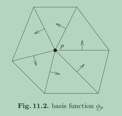
Now consider the vertex basis $\boldsymbol{\phi}_p$ on some element $T\in\omega_p$, denote the joint edge of $p$ as $e_1$ and $e_2$ we have
\[\operatorname{div} \boldsymbol{\phi}_p\big\vert_T = \frac{1}{|e_1|} \nabla \psi_{e_1} \cdot \boldsymbol{n}_{e_1} + \frac{1}{|e_2|} \nabla \psi_{e_2} \cdot \boldsymbol{n}_{e_2}.\]
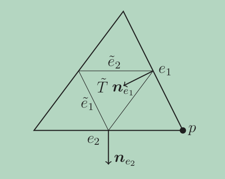
Refer to the figure above, $\nabla \psi_{e_1}$ is the inner normal vector of $\tilde{e}_1$ with respect to the triangle $\tilde{T}$, denote the inner normal vector as $\boldsymbol{\nu}_{\tilde{e}_1}$ then we have
\[\nabla \psi_{e_1} = \frac{1}{2|\tilde{T}|} \boldsymbol{\nu}_{\tilde{e}_1} = -\frac{1}{2|\tilde{T}|} |\tilde{e}_1| \boldsymbol{n}_{e_1} = -\frac{|e_1|}{|T|}\boldsymbol{n}_{e_1},\]therefore
\[\frac{1}{|e_1|} \nabla \psi_{e_1} \cdot \boldsymbol{n}_{e_1} = -\frac{1}{|T|}.\]Similarly, we have
\[\frac{1}{|e_2|} \nabla \psi_{e_2} \cdot \boldsymbol{n}_{e_2} = \frac{1}{|T|},\]hence
\[\operatorname{div} \boldsymbol{\phi}_p\big|_T = 0.\]Part 2: write a vector as the linear combination of basis functions
Now for $\forall M$ which is the midpoint of an edge $e_i$ in this patch, consider $T^+$ and $T^-$, where $\omega_e = T^+ \cup T^-$. For the space $\boldsymbol{V}_h^* $ in which the functions are continuous at $M$, consider $\forall \boldsymbol{w} \in \boldsymbol{V}_h^*$, $\boldsymbol{w}(M)$ is a constant vector, hence we could decompose $\boldsymbol{w}$ into two orthogonal vectors in the directions of $\boldsymbol{t}_e$ and $\boldsymbol{n}_e$, respectively. At point $M$ we have:
\[\boldsymbol{w}(M) = (\boldsymbol{w}\cdot\boldsymbol{t}_e)\boldsymbol{t}_e + (\boldsymbol{w}\cdot\boldsymbol{n}_e)\boldsymbol{n}_e.\]This is true because at point $M$ we could express $\boldsymbol{w} = |\boldsymbol{w}|\boldsymbol{\xi}$, where $\boldsymbol{\xi}$ is the unit vector in $\boldsymbol{w}$’s direction, denote the angle between $\boldsymbol{w}$ and $\boldsymbol{t}_e$ as $\theta$,
\[\boldsymbol{\xi} = \boldsymbol{t}_e\cos \theta + \boldsymbol{n}_e\sin \theta= \boldsymbol{t}_e \left(\frac{\boldsymbol{w}}{|\boldsymbol{w}|}\cdot\boldsymbol{t}_e\right) + \boldsymbol{n}_e\left(\frac{\boldsymbol{w}}{|\boldsymbol{w}|}\cdot\boldsymbol{n}_e\right).\]It is easy to see that $\boldsymbol{\xi}\cdot \boldsymbol{\xi} = 1$ since $\boldsymbol{t}_e$ and $\boldsymbol{n}_e$ are orthogonal. Now at $M$ we know $\psi_e = 1$, hence we could express at $M$:
\[\boldsymbol{w} = (\boldsymbol{w}\cdot\boldsymbol{t}_e)\psi_e\boldsymbol{t}_e + (\boldsymbol{w}\cdot\boldsymbol{n}_e)\psi_e\boldsymbol{n}_e.\]Since for all other four midpoints within the $\omega_e = T^+ \cup T^-$, the basis functions $\psi_{e’}$ for $e’\subset \partial \omega_e$ are all zero at $M$, and linear within the triangle, any linear vector that could be decomposed this way at $M$ bears the same continuity with two basis function $\psi_e \boldsymbol{t}_e$ and $\psi_e \boldsymbol{n}_e $ at the same edge. Other edge bases vanish at $M$. In other words, the linear vector could be written in this way is continuous at $M$.
Now locally within any element $T$ that has edge $e_1$, $e_2$, and $e_3$, with midpoints $M_1$, $M_2$ and $M_3$, $\forall x\in T $, for any linear vector $\boldsymbol{w}$ decompose
\[\begin{aligned} \boldsymbol{w}(x) &= \boldsymbol{w}(\psi_{e_1}(x)M_1 + \psi_{e_2}(x)M_2 + \psi_{e_3}(x)M_3 ) \\ &= \psi_{e_1}(x) \boldsymbol{w}(M_1) + \psi_{e_2}(x) \boldsymbol{w}(M_2) + \psi_{e_3}(x) \boldsymbol{w}(M_3) \end{aligned}\]for each $ \psi_{e_j}(x)\boldsymbol{w}(M_j) $ which is a constant at $ x $, decompose it in the same fashion as before along the direction of $\boldsymbol{t}_{e_j}$ and $ \boldsymbol{n}_{e_j} $. Hence $\forall \boldsymbol{w}\in \boldsymbol{V}_h^*$, globally we could write it as
\[\boldsymbol{w} = \sum_{e\in \mathcal{E}_h} \Bigl((\boldsymbol{w}(M_e)\cdot \boldsymbol{t}_e) \boldsymbol{\phi}_e + (\boldsymbol{w}(M_e)\cdot \boldsymbol{n}_e) \boldsymbol{\eta}_e \Bigr)\]where $\boldsymbol{\phi}_e = \psi_e \boldsymbol{t}_e$ and $\boldsymbol{\eta}_e = \psi_e \boldsymbol{n}_e$. Moreover, $\boldsymbol{\phi}_e\perp \boldsymbol{\eta}_e$, i.e., they are linearly independent. Now we have shown $\{\boldsymbol{\phi}_e\}$ and $\{\boldsymbol{\eta}_e\}$ form a set of basis functions for $\boldsymbol{V}^*_h$.
Part 3: more on the divergence-freeness
For the divergence zero subspace, we have already shown
\[\operatorname{div}_h \boldsymbol{\phi}_e = 0.\]It suffices to show that $\forall \boldsymbol{v}$ such that
\[\boldsymbol{v} = \sum_{e\in \mathcal{E}_h} (\boldsymbol{w}(M_e)\cdot \boldsymbol{n}_e) \boldsymbol{\eta}_e = \sum_{e\in \mathcal{E}_h} b_e \boldsymbol{\eta}_e\in \boldsymbol{V}^*_h\]of which $\operatorname{div}_h\boldsymbol{v} = 0$. This $\boldsymbol{v}$ can be written as
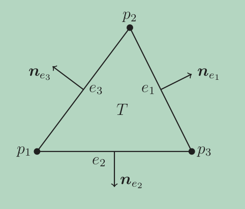
\[\boldsymbol{v} = \sum_{p\in \mathcal{V}_h} b_p \boldsymbol{\phi}_p.\]Now consider within an arbitrary element $ T\subset \omega_e $, and assign a fixed unit outer normal vector to each edge of $T$ as in the following figure we have:
\[\begin{aligned} 0 = \operatorname{div}_h\boldsymbol{v}\Big|_T &= \sum_{e\in \mathcal{E}_h} \Bigl( (\boldsymbol{v}(M_e)\cdot \boldsymbol{n}_e) \operatorname{div}_h(\boldsymbol{\eta}_e) + \nabla_h (\boldsymbol{v}(M_e)\cdot \boldsymbol{n}_e) \boldsymbol{\eta}_e \Bigr) \\ 0&= \sum_{e\subset \partial T} (\boldsymbol{v}(M_e)\cdot \boldsymbol{n}_e) (\nabla \psi_e \cdot \boldsymbol{n}_e) \quad \\ 0&= (\boldsymbol{v}(M_1)\cdot \boldsymbol{n}_{e_1}) \frac{|e_1|}{|T|} + (\boldsymbol{v}(M_2)\cdot \boldsymbol{n}_{e_2}) \frac{|e_2|}{|T|} + (\boldsymbol{v}(M_3)\cdot \boldsymbol{n}_{e_3}) \frac{|e_3|}{|T|} \end{aligned}\]rewriting above using the coefficients we have
\[b_{e_1}|e_1| + b_{e_2}|e_2| + b_{e_3}|e_3| = 0. \tag{1}\label{divfree}\]
Therefore, as long as the coefficients of edge basis functions satisfy above relation, the vector field is divergence free within this element $T$.
Now consider the linear vector field $\boldsymbol{u} = \sum_{p\in \mathcal{V}_h} b_p \boldsymbol{\phi}_p$ within $T$, in the following equation we would like to rewrite $\boldsymbol{\phi}_p$’s counterclockwise normal vector aligning with the local unit outward normal, and we have:
\[\begin{aligned} \boldsymbol{u} &= b_{p_1} \boldsymbol{\phi}_{p_1} + b_{p_2} \boldsymbol{\phi}_{p_2} + b_{p_3} \boldsymbol{\phi}_{p_3} \\ &= b_{p_1} \Bigl(\frac{1}{|e_3|}\boldsymbol{\eta}_{e_3} - \frac{1}{|e_2|}\boldsymbol{\eta}_{e_2} \Bigr) + b_{p_2} \Bigl(\frac{1}{|e_1|}\boldsymbol{\eta}_{e_1} - \frac{1}{|e_3|}\boldsymbol{\eta}_{e_3}\Bigr) + b_{p_3} \Bigl(\frac{1}{|e_2|}\boldsymbol{\eta}_{e_2} - \frac{1}{|e_1|}\boldsymbol{\eta}_{e_1} \Bigr) \\ &= \frac{1}{|e_1|}(b_{p_2} - b_{p_3})\boldsymbol{\eta}_{e_1} + \frac{1}{|e_2|}(b_{p_3} - b_{p_1})\boldsymbol{\eta}_{e_2} + \frac{1}{|e_3|}(b_{p_1} - b_{p_2})\boldsymbol{\eta}_{e_3} \\ &:= b_{e_1}\boldsymbol{\eta}_{e_1} + b_{e_2}\boldsymbol{\eta}_{e_2} + b_{e_3}\boldsymbol{\eta}_{e_3} \end{aligned}\]It is obvious that here the coefficients satisfy \eqref{divfree}. Also the converse is also true, for a divergence free vector
\[\boldsymbol{u} = b_{e_1}\boldsymbol{\eta}_{e_1} + b_{e_2}\boldsymbol{\eta}_{e_2} + b_{e_3}\boldsymbol{\eta}_{e_3}\]within element $T$, by\eqref{divfree} we have
\[\begin{aligned} \boldsymbol{u} &= b_{e_1}\boldsymbol{\eta}_{e_1} + b_{e_2}\boldsymbol{\eta}_{e_2} - \frac{1}{|e_3|} (b_{e_1}|e_1| + b_{e_2}|e_2|)\boldsymbol{\eta}_{e_3} \\ &= b_{e_1}|e_1|\bigl(\frac{1}{|e_1|}\boldsymbol{\eta}_{e_1} - \frac{1}{|e_3|}\boldsymbol{\eta}_{e_3} \bigr) + b_{e_2}|e_2|\bigl(\frac{1}{|e_2|}\boldsymbol{\eta}_{e_2} - \frac{1}{|e_3|}\boldsymbol{\eta}_{e_3} \bigr) \\ &= b_{p_2} \boldsymbol{\phi}_{p_2} + b_{p_1}\boldsymbol{\phi}_{p_1} \end{aligned}\]or a linear combination of $\boldsymbol{\phi}_{p_3}$ and $\boldsymbol{\phi}_{p_2}$, or $\boldsymbol{\phi}_{p_3}$ and $\boldsymbol{\phi}_{p_1}$ due to relation \eqref{divfree}. Hence here we proved that locally within each element $T$, any divergence free linear vector field could be written as the linear combination of the $\{\boldsymbol{\phi}_e\}_{e\subset \partial T}$ and $\{\boldsymbol{\phi}_p\}_{p\in \mathcal{V}_T}$.
Part 4: how does the global continuity condition work?
Now we would like to prove globally glued together with the continuity condition, $\boldsymbol{\phi}_p$ will bear the following form globally:
\[\boldsymbol{\phi}_p = \sum^l_{i=1} \frac{1}{|e_i|} \psi_{e_i} \boldsymbol{n}_{e_i}\]Consider the vertex $p$, the edge $e_1$, $e_2$, and $e_3$, two elements $T_1$ and $T_2$, unit normal for each edge fixed as in the following figure, and $\boldsymbol{\eta}_{e_i} = \psi_{e_i}\boldsymbol{n}_{e_i}$:
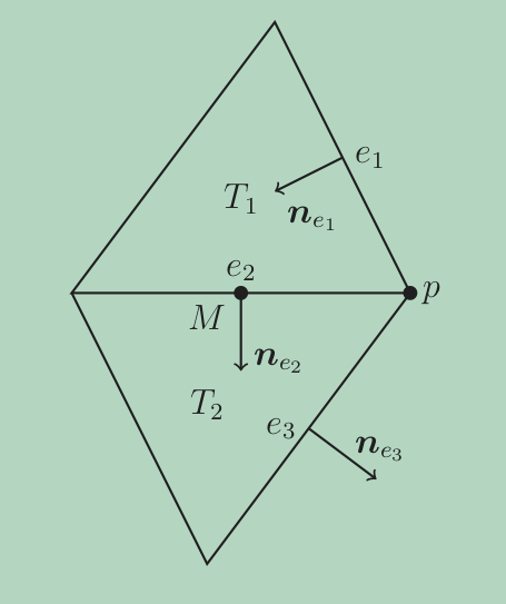
We already knew that locally in $T_1$:
\[\boldsymbol{\phi}_p\big|_{T_1} = \frac{1}{|e_1|}\, \boldsymbol{\eta}_{e_1}\big|_{T_1} + \frac{1}{|e_2|} \,\boldsymbol{\eta}_{e_2}\big|_{T_1}\]clearly coefficients satisfy \eqref{divfree}. Similarly, we could get
\[\boldsymbol{\phi}_p\big|_{T_2} = \frac{1}{|e_2|} \,\boldsymbol{\eta}_{e_2}\big|_{T_2} + \frac{1}{|e_3|} \, \boldsymbol{\eta}_{e_3}\big|_{T_2}\]Consider any $\boldsymbol{u}$ that is divergence free within $T_1$ and $T_2$, that
\[\boldsymbol{u}\big|_{T_1} = a_1 \boldsymbol{\phi}_p\big|_{T_1}, \quad \boldsymbol{u}\big|_{T_2} = a_2 \boldsymbol{\phi}_p\big|_{T_2}\]and while continuous at $M$:
\[\lim_{x\to M,x\in T_1} \boldsymbol{u}= \frac{a_1}{|e_2|} \boldsymbol{n}_{e_2} = \lim_{x\to M,x\in T_2} \boldsymbol{u} = \frac{a_2}{|e_2|} \boldsymbol{n}_{e_2}\]this implies $a_1 = a_2$, i.e., the coefficient for each $\boldsymbol{\phi}_{p}\big|_{T_i}$ should be the same when marching counterclockwisely around this patch, where $T_i \subset \omega_p$ is an element within this patch. Together with last part, this implies
\[\{\boldsymbol{\phi}_p\} = \{\boldsymbol{v}: \boldsymbol{v} = \sum_{e\in \mathcal{T}_h} b_e\boldsymbol{\eta}_e\}\bigcap \{\boldsymbol{v}: \operatorname{div}_h \boldsymbol{v} = 0\}\]Therefore, $\{\boldsymbol{\phi}_e\}$ and $\{\boldsymbol{\phi}_p\}$ are shown to be the basis functions for the space
\(\boldsymbol{W}_h = \{\boldsymbol{v}\in \boldsymbol{V}_h^*: \operatorname{div}_h \boldsymbol{v} = 0\}\).
A final remark
Notice for general vector field $\boldsymbol{u}$, the nodal interpolation of it onto $\boldsymbol{V}^*_h$ is
\[\operatorname{I}_{\boldsymbol{V}^*_h}\boldsymbol{u} = \sum_{T\in \mathcal{T}_h}\sum_{e\subset \partial T} \Bigl((\boldsymbol{u},\boldsymbol{\phi}_e)_T \boldsymbol{\phi}_e + (\boldsymbol{u}, \boldsymbol{\eta}_e)_T \boldsymbol{\eta}_e \Bigr).\]and this projection does not coincide with the “nodal” interpolation of linear vector field $\boldsymbol{u}$ using pointwise value as coefficient, since
\[\begin{aligned} (\boldsymbol{u},\boldsymbol{\phi}_e)_T &= \int_T \boldsymbol{u} \cdot \boldsymbol{t}_e \psi_e \,dx \\ &= \frac{|e|}{2|T|} \int_T \boldsymbol{u} \cdot \nabla^{\perp} \psi_e^2 \,dx \\ &= \frac{|e|}{2|T|} \int_T \nabla\times \boldsymbol{u} \,\psi_e^2\,dx + \frac{|e|}{2|T|} \int_{\partial K} \boldsymbol{u}\cdot \boldsymbol{t} \psi_e^2 \,ds. \end{aligned}\]References
-
Brenner, S.C. and Scott, R. (2008) The mathematical theory of finite element methods. Springer.
Comments